#import os
from sympy import *
import numpy as np
from tabulate import tabulate
from scipy import signal
import matplotlib.pyplot as plt
import pandas as pd
import SymMNA
from IPython.display import display, Markdown, Math, Latex
init_printing()12 Thevenin Equivalent Circuit
The Thevenin equivalent circuit is the reduction of a linear circuit to a single source and impedance and is based on Thevenin’s Theorem. The history of the Thévenin equivalent circuit is a classic case of scientific double discovery. While it bears the name of a French telegraph engineer, it was actually first formulated thirty years earlier by Hermann von Helmholtz in 1853.
Helmholtz was an expert in many fields, including physiology. He was trying to understand the distribution of electrical currents in animal tissue (what was then called animal electricity). He realized that no matter how complex a network of conductors and sources was, it would behave toward an external load like a single conductor in series with a single electromotive force (voltage). Because Helmholtz published his findings in a physics journal focused on physiology and general physics (Annalen der Physik und Chemie), his work remained largely unknown to the emerging field of electrical engineering for decades.
Thirty years later, Léon Charles Thévenin, a young engineer with the French National Post and Telegraph organization, independently arrived at the same conclusion. Thévenin was teaching at the École Supérieure de Télégraphie and wanted to simplify the analysis of complex telegraph networks. He was looking for a way to extend Ohm’s Law to more complicated systems. In 1883, he published his theorem in the journal Annales Télégraphiques under the title Sur un nouveau théorème d’électricité dynamique (On a new theorem of dynamic electricity). Unlike Helmholtz’s earlier work, Thévenin’s proof was written specifically for the engineering community. It was more practical and included clear steps for calculation, leading to its widespread adoption in the late 19th century.
The theorem states that any linear electrical network with voltage/current sources and resistances can be replaced at its terminals by an equivalent circuit consisting of a single voltage source and a single series resistor. \(V_{th}\) is the open-circuit voltage at the terminals and \(R_{th}\) is the resistance measured back into the terminals with all independent sources turned off (voltage sources shorted, current sources opened).
For many years, the theorem was known only as “Thévenin’s Theorem.” It wasn’t until the mid-20th century that Hans Ferdinand Mayer pointed out Helmholtz’s earlier work. Consequently, some modern textbooks refer to it as the Helmholtz-Thévenin Theorem to give credit to both inventors.
While it was originally designed for telegraphy, Thévenin’s Theorem is now a fundamental tool in everything from green energy to high-speed computing. Its primary modern value lies in abstraction - allowing engineers to ignore the internal complexity of a large system and focus only on how it interacts with a single component.
12.1 Example Problem
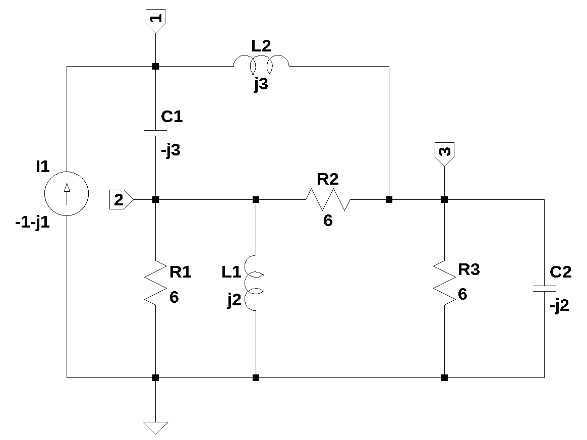
The example used in this chapter is a problem from Johnson, Hilburn, and Johnson (1978), problem 11.25. The student is asked to: Replace the circuit to the left of terminals a-b by its Thevenin equivalent and find \(V\). The schematic for the problem is shown in Figure 12.1.
The Python libraries of SimPy and NumPy are used to perform the math in the proposed solution. The schematic shown below was drawn using LTspice and the nodes were numbered. Terminals a and b are also labeled. The circuit given in the textbook does not include a reference node. The node at the bottom of the schematic seemed like a convenient location for the reference since we are asked to provide \(V\).
The following steps are used to find the Thevenin equivalent circuit:
- Obtain the circuit’s netlist, either by hand or exported from the schematic. Make any edits to the netlist as needed.
- Remove the load, in this case \(R_3\) and \(C_2\), from the netlist.
- Find the voltage \(V_{oc}\) at terminals a and b.
- Find the short circuit current, \(I_{sc}\) at the terminals a and b.
- Calculate \(R_{th}\) from \(V_{oc}\) and \(I_{sc}\).
Having drawn the circuit in LTspice, the following netlist was exported as a text file.
R1 2 0 6
R2 3 2 6
R3 0 3 6
L1 2 0 j2
L2 1 3 j3
C1 1 2 -j3
C2 3 0 -j2
I1 0 1 -1-j1
The component values for the inductors and capacitors are complex as well as the value of the current source. It is assumed that the impedance of the inductors and capacitors are at a frequency of \(\omega=1\). So accordingly, the values in the net list used by the Python code to generate the network equations has been adjusted as follows:
R1 2 0 6
R2 3 2 6
R3 0 3 6
L1 2 0 2
L2 1 3 3
C1 1 2 0.3333
C2 3 0 0.5
I1 0 1 1
The following Python libraries are included in the JupyterLab notebook.
Removing \(R_3\) and \(C_2\) by commenting out those lines in the netlist, this gives \(V_{oc} = v_3\). The net list is:
I1 0 1 1
R1 2 0 6
R2 3 2 6
*R3 0 3 6
L1 2 0 2
L2 1 3 3
C1 1 2 0.3333
*C2 3 0 0.5
Load the net list string into the variable.
net_list = '''
I1 0 1 1
R1 2 0 6
R2 3 2 6
*R3 0 3 6
L1 2 0 2
L2 1 3 3
C1 1 2 0.3333
*C2 3 0 0.5
'''
Call the symbolic modified nodal analysis function to obtain the network matrices.
report, network_df, i_unk_df, A, X, Z = SymMNA.smna(net_list)Put X and Z into Matrix type, build the equations and use markdown to display the equations.
# Put matrices into SymPy
X = Matrix(X)
Z = Matrix(Z)

NE_sym = Eq(A*X,Z)

# turn the free symbols into SymPy variables.
var(str(NE_sym.free_symbols).replace('{','').replace('}',''))

# construct a dictionary of element values
element_values = SymMNA.get_part_values(network_df)

temp = ''
for i in range(len(X)):
    temp += '${:s}$<br>'.format(latex(Eq((A*X)[i:i+1][0],Z[i])))

Markdown(temp)
\(C_{1} s v_{1} - C_{1} s v_{2} + I_{L2} = I_{1}\)
\(- C_{1} s v_{1} + I_{L1} + v_{2} \left(C_{1} s + \frac{1}{R_{2}} + \frac{1}{R_{1}}\right) - \frac{v_{3}}{R_{2}} = 0\)
\(- I_{L2} - \frac{v_{2}}{R_{2}} + \frac{v_{3}}{R_{2}} = 0\)
\(- I_{L1} L_{1} s + v_{2} = 0\)
\(- I_{L2} L_{2} s + v_{1} - v_{3} = 0\)
Generate and display the symbolic solution.
U_sym = solve(NE_sym,X)

temp = ''
for i in U_sym.keys():
    temp += '${:s} = {:s}$<br>'.format(latex(i),latex(U_sym[i]))

Markdown(temp)
\(v_{1} = \frac{C_{1} I_{1} L_{1} L_{2} R_{1} s^{3} + C_{1} I_{1} L_{1} R_{1} R_{2} s^{2} + I_{1} L_{1} L_{2} s^{2} + I_{1} L_{1} R_{1} s + I_{1} L_{1} R_{2} s + I_{1} L_{2} R_{1} s + I_{1} R_{1} R_{2}}{C_{1} L_{1} L_{2} s^{3} + C_{1} L_{1} R_{2} s^{2} + C_{1} L_{2} R_{1} s^{2} + C_{1} R_{1} R_{2} s + L_{1} s + R_{1}}\)
\(v_{2} = \frac{I_{1} L_{1} R_{1} s}{L_{1} s + R_{1}}\)
\(v_{3} = \frac{C_{1} I_{1} L_{1} L_{2} R_{1} s^{3} + C_{1} I_{1} L_{1} R_{1} R_{2} s^{2} + I_{1} L_{1} R_{1} s + I_{1} L_{1} R_{2} s + I_{1} R_{1} R_{2}}{C_{1} L_{1} L_{2} s^{3} + C_{1} L_{1} R_{2} s^{2} + C_{1} L_{2} R_{1} s^{2} + C_{1} R_{1} R_{2} s + L_{1} s + R_{1}}\)
\(I_{L1} = \frac{I_{1} R_{1}}{L_{1} s + R_{1}}\)
\(I_{L2} = \frac{I_{1}}{C_{1} L_{2} s^{2} + C_{1} R_{2} s + 1}\)
To solve numerically, replace symbols with the element values and the Laplace variable, s, with \(j\omega\) where \(\omega=1\). The value for \(C_1\) is replaced by the fraction \(1/3\) so that the exact value can be used in the numerical calculations.
NE = NE_sym.subs({C1:1/3, s:1j, I1:-1-1j})
NE = NE.subs(element_values)

temp = ''
for i in range(shape(NE.lhs)[0]):
    temp += '${:s} = {:s}$<br>'.format(latex(NE.rhs[i]),latex(NE.lhs[i]))

Markdown(temp)
\(-1.0 - 1.0 i = I_{L2} + 0.333333333333333 i v_{1} - 0.333333333333333 i v_{2}\)
\(0 = I_{L1} - 0.333333333333333 i v_{1} + v_{2} \cdot \left(0.333333333333333 + 0.333333333333333 i\right) - 0.166666666666667 v_{3}\)
\(0 = - I_{L2} - 0.166666666666667 v_{2} + 0.166666666666667 v_{3}\)
\(0 = - 2.0 i I_{L1} + v_{2}\)
\(0 = - 3.0 i I_{L2} + v_{1} - v_{3}\)
Solving the system of equations for the open circuit voltage at node \(v_3\).
Voc = solve(NE,X)[v3]
Voc
\(\displaystyle -1.8 + 0.6 i\)
Find the short circuit current, \(I_{sc}\) by removing \(C_2\) and \(R_3\), setting node 3 to zero and finding the current in \(L_2\) and \(R_2\). The new net list is:
net_list = '''
I1 0 1 1
R1 2 0 6
R2 0 2 6
L1 2 0 2
L2 1 0 3
C1 1 2 0.3333
'''
Call the symbolic modified nodal analysis function to get the MNA matrices.
report, network_df, i_unk_df, A, X, Z = SymMNA.smna(net_list)Put X and Z into Matrix type, build the equations and use markdown to display the equations.
# Put matrices into SymPy
X = Matrix(X)
Z = Matrix(Z)

NE_sym = Eq(A*X,Z)

# turn the free symbols into SymPy variables.
var(str(NE_sym.free_symbols).replace('{','').replace('}',''))

# construct a dictionary of element values
element_values = SymMNA.get_part_values(network_df)

temp = ''
for i in range(len(X)):
    temp += '${:s}$<br>'.format(latex(Eq((A*X)[i:i+1][0],Z[i])))

Markdown(temp)
\(C_{1} s v_{1} - C_{1} s v_{2} + I_{L2} = I_{1}\)
\(- C_{1} s v_{1} + I_{L1} + v_{2} \left(C_{1} s + \frac{1}{R_{2}} + \frac{1}{R_{1}}\right) = 0\)
\(- I_{L1} L_{1} s + v_{2} = 0\)
\(- I_{L2} L_{2} s + v_{1} = 0\)
Find the symbolic solution and display the solution.
U_sym = solve(NE_sym,X)

temp = ''
for i in U_sym.keys():
    temp += '${:s} = {:s}$<br>'.format(latex(i),latex(U_sym[i]))

Markdown(temp)
\(v_{1} = \frac{C_{1} I_{1} L_{1} L_{2} R_{1} R_{2} s^{3} + I_{1} L_{1} L_{2} R_{1} s^{2} + I_{1} L_{1} L_{2} R_{2} s^{2} + I_{1} L_{2} R_{1} R_{2} s}{C_{1} L_{1} L_{2} R_{1} s^{3} + C_{1} L_{1} L_{2} R_{2} s^{3} + C_{1} L_{1} R_{1} R_{2} s^{2} + C_{1} L_{2} R_{1} R_{2} s^{2} + L_{1} R_{1} s + L_{1} R_{2} s + R_{1} R_{2}}\)
\(v_{2} = \frac{C_{1} I_{1} L_{1} L_{2} R_{1} R_{2} s^{3}}{C_{1} L_{1} L_{2} R_{1} s^{3} + C_{1} L_{1} L_{2} R_{2} s^{3} + C_{1} L_{1} R_{1} R_{2} s^{2} + C_{1} L_{2} R_{1} R_{2} s^{2} + L_{1} R_{1} s + L_{1} R_{2} s + R_{1} R_{2}}\)
\(I_{L1} = \frac{C_{1} I_{1} L_{2} R_{1} R_{2} s^{2}}{C_{1} L_{1} L_{2} R_{1} s^{3} + C_{1} L_{1} L_{2} R_{2} s^{3} + C_{1} L_{1} R_{1} R_{2} s^{2} + C_{1} L_{2} R_{1} R_{2} s^{2} + L_{1} R_{1} s + L_{1} R_{2} s + R_{1} R_{2}}\)
\(I_{L2} = \frac{C_{1} I_{1} L_{1} R_{1} R_{2} s^{2} + I_{1} L_{1} R_{1} s + I_{1} L_{1} R_{2} s + I_{1} R_{1} R_{2}}{C_{1} L_{1} L_{2} R_{1} s^{3} + C_{1} L_{1} L_{2} R_{2} s^{3} + C_{1} L_{1} R_{1} R_{2} s^{2} + C_{1} L_{2} R_{1} R_{2} s^{2} + L_{1} R_{1} s + L_{1} R_{2} s + R_{1} R_{2}}\)
The current through \(R_2\) and \(L_2\) can be expressed symbolically as:
U_sym[v2]/R2 + U_sym[I_L2]\(\displaystyle \frac{C_{1} I_{1} L_{1} L_{2} R_{1} s^{3}}{C_{1} L_{1} L_{2} R_{1} s^{3} + C_{1} L_{1} L_{2} R_{2} s^{3} + C_{1} L_{1} R_{1} R_{2} s^{2} + C_{1} L_{2} R_{1} R_{2} s^{2} + L_{1} R_{1} s + L_{1} R_{2} s + R_{1} R_{2}} + \frac{C_{1} I_{1} L_{1} R_{1} R_{2} s^{2} + I_{1} L_{1} R_{1} s + I_{1} L_{1} R_{2} s + I_{1} R_{1} R_{2}}{C_{1} L_{1} L_{2} R_{1} s^{3} + C_{1} L_{1} L_{2} R_{2} s^{3} + C_{1} L_{1} R_{1} R_{2} s^{2} + C_{1} L_{2} R_{1} R_{2} s^{2} + L_{1} R_{1} s + L_{1} R_{2} s + R_{1} R_{2}}\)
After substituting the numerical values for the comments, we can display the network equations.
NE = NE_sym.subs({C1:1/3, s:1j, I1:-1-1j})
NE = NE.subs(element_values)

temp = ''
for i in range(shape(NE.lhs)[0]):
    temp += '${:s} = {:s}$<br>'.format(latex(NE.rhs[i]),latex(NE.lhs[i]))

Markdown(temp)
\(-1.0 - 1.0 i = I_{L2} + 0.333333333333333 i v_{1} - 0.333333333333333 i v_{2}\)
\(0 = I_{L1} - 0.333333333333333 i v_{1} + v_{2} \cdot \left(0.333333333333333 + 0.333333333333333 i\right)\)
\(0 = - 2.0 i I_{L1} + v_{2}\)
\(0 = - 3.0 i I_{L2} + v_{1}\)
The equations are easily solved by SymPy.
U = solve(NE,X)The short circuit current is the sum of the currents through \(R_6\).
Isc = U[v2]/element_values[R2] + U[I_L2]
Isc
\(\displaystyle 1.0 i\)
The Thevenin resistance is \(\frac{V_{oc}}{I_{sc}}\)
Zth = simplify(Voc/Isc)
Zth
\(\displaystyle 0.6 + 1.8 i\)
\(V_{oc}\) along with \(Z_{th}\) are the components of the Thevenin equivalent circuit.
The second part of the problem asks us to find \(v_3\) using the Thevenin equivalent circuit. The load attached to the Thevenin equivalent circuit is the parallel combination of \(R_3\) and \(C_2\).
\(Z = \frac{1}{\frac{1}{R_3}+\frac{1}{C_2}}\)
The load \(Z\) is the parallel combination of \(R_3 = 6\) and \(C_2 = -j2\).
Z = (1)/(1/(6)+1/(-2j))
Z(0.6-1.7999999999999998j)Using the values for \(V_{oc}\) and \(Z_{th}\) obtained above, we write the equation for V3 as a voltage divider and have SymPy simplify the result.
simplify(Z*Voc/(Zth+Z))\(\displaystyle 4.62592926927148 \cdot 10^{-16} + 3.0 i\)
We can get SymPy to ignore small numbers by using the round function set to 3 digits.
simplify(Z*Voc/(Zth+Z)).round(3)\(\displaystyle 3.0 i\)
12.1.1 Find \(v_3\) using the complete circuit
We can check the answer for \(v_3\), by solving the equations for the complete circuit. The net list is:
net_list = '''
I1 0 1 1
R1 2 0 6
R2 3 2 6
R3 0 3 6
L1 2 0 2
L2 1 3 3
C1 1 2 0.3333
C2 3 0 0.5
'''
Call the symbolic modified nodal analysis function to generate the MNA matrices.
report, network_df, i_unk_df, A, X, Z = SymMNA.smna(net_list)The matrices are converted to SymPy types and the symbolic network equations are displayed using markdown.
# Put matrices into SymPy
X = Matrix(X)
Z = Matrix(Z)

NE_sym = Eq(A*X,Z)

# turn the free symbols into SymPy variables.
var(str(NE_sym.free_symbols).replace('{','').replace('}',''))

# construct a dictionary of element values
element_values = SymMNA.get_part_values(network_df)

temp = ''
for i in range(len(X)):
    temp += '${:s}$<br>'.format(latex(Eq((A*X)[i:i+1][0],Z[i])))

Markdown(temp)
\(C_{1} s v_{1} - C_{1} s v_{2} + I_{L2} = I_{1}\)
\(- C_{1} s v_{1} + I_{L1} + v_{2} \left(C_{1} s + \frac{1}{R_{2}} + \frac{1}{R_{1}}\right) - \frac{v_{3}}{R_{2}} = 0\)
\(- I_{L2} + v_{3} \left(C_{2} s + \frac{1}{R_{3}} + \frac{1}{R_{2}}\right) - \frac{v_{2}}{R_{2}} = 0\)
\(- I_{L1} L_{1} s + v_{2} = 0\)
\(- I_{L2} L_{2} s + v_{1} - v_{3} = 0\)
Use SymPy to find the symbolic solution.
U_sym = solve(NE_sym,X)Display the symbolic solution.
temp = ''
for i in U_sym.keys():
    temp += '${:s} = {:s}$<br>'.format(latex(i),latex(U_sym[i]))

Markdown(temp)
\(v_{1} = \frac{C_{1} C_{2} I_{1} L_{1} L_{2} R_{1} R_{2} R_{3} s^{4} + C_{1} I_{1} L_{1} L_{2} R_{1} R_{2} s^{3} + C_{1} I_{1} L_{1} L_{2} R_{1} R_{3} s^{3} + C_{1} I_{1} L_{1} R_{1} R_{2} R_{3} s^{2} + C_{2} I_{1} L_{1} L_{2} R_{1} R_{3} s^{3} + C_{2} I_{1} L_{1} L_{2} R_{2} R_{3} s^{3} + C_{2} I_{1} L_{2} R_{1} R_{2} R_{3} s^{2} + I_{1} L_{1} L_{2} R_{1} s^{2} + I_{1} L_{1} L_{2} R_{2} s^{2} + I_{1} L_{1} L_{2} R_{3} s^{2} + I_{1} L_{1} R_{1} R_{3} s + I_{1} L_{1} R_{2} R_{3} s + I_{1} L_{2} R_{1} R_{2} s + I_{1} L_{2} R_{1} R_{3} s + I_{1} R_{1} R_{2} R_{3}}{C_{1} C_{2} L_{1} L_{2} R_{1} R_{3} s^{4} + C_{1} C_{2} L_{1} L_{2} R_{2} R_{3} s^{4} + C_{1} C_{2} L_{1} R_{1} R_{2} R_{3} s^{3} + C_{1} C_{2} L_{2} R_{1} R_{2} R_{3} s^{3} + C_{1} L_{1} L_{2} R_{1} s^{3} + C_{1} L_{1} L_{2} R_{2} s^{3} + C_{1} L_{1} L_{2} R_{3} s^{3} + C_{1} L_{1} R_{1} R_{2} s^{2} + C_{1} L_{1} R_{2} R_{3} s^{2} + C_{1} L_{2} R_{1} R_{2} s^{2} + C_{1} L_{2} R_{1} R_{3} s^{2} + C_{1} R_{1} R_{2} R_{3} s + C_{2} L_{1} R_{1} R_{3} s^{2} + C_{2} L_{1} R_{2} R_{3} s^{2} + C_{2} R_{1} R_{2} R_{3} s + L_{1} R_{1} s + L_{1} R_{2} s + L_{1} R_{3} s + R_{1} R_{2} + R_{1} R_{3}}\)
\(v_{2} = \frac{C_{1} C_{2} I_{1} L_{1} L_{2} R_{1} R_{2} R_{3} s^{4} + C_{1} I_{1} L_{1} L_{2} R_{1} R_{2} s^{3} + C_{1} I_{1} L_{1} L_{2} R_{1} R_{3} s^{3} + C_{1} I_{1} L_{1} R_{1} R_{2} R_{3} s^{2} + I_{1} L_{1} R_{1} R_{3} s}{C_{1} C_{2} L_{1} L_{2} R_{1} R_{3} s^{4} + C_{1} C_{2} L_{1} L_{2} R_{2} R_{3} s^{4} + C_{1} C_{2} L_{1} R_{1} R_{2} R_{3} s^{3} + C_{1} C_{2} L_{2} R_{1} R_{2} R_{3} s^{3} + C_{1} L_{1} L_{2} R_{1} s^{3} + C_{1} L_{1} L_{2} R_{2} s^{3} + C_{1} L_{1} L_{2} R_{3} s^{3} + C_{1} L_{1} R_{1} R_{2} s^{2} + C_{1} L_{1} R_{2} R_{3} s^{2} + C_{1} L_{2} R_{1} R_{2} s^{2} + C_{1} L_{2} R_{1} R_{3} s^{2} + C_{1} R_{1} R_{2} R_{3} s + C_{2} L_{1} R_{1} R_{3} s^{2} + C_{2} L_{1} R_{2} R_{3} s^{2} + C_{2} R_{1} R_{2} R_{3} s + L_{1} R_{1} s + L_{1} R_{2} s + L_{1} R_{3} s + R_{1} R_{2} + R_{1} R_{3}}\)
\(v_{3} = \frac{C_{1} I_{1} L_{1} L_{2} R_{1} R_{3} s^{3} + C_{1} I_{1} L_{1} R_{1} R_{2} R_{3} s^{2} + I_{1} L_{1} R_{1} R_{3} s + I_{1} L_{1} R_{2} R_{3} s + I_{1} R_{1} R_{2} R_{3}}{C_{1} C_{2} L_{1} L_{2} R_{1} R_{3} s^{4} + C_{1} C_{2} L_{1} L_{2} R_{2} R_{3} s^{4} + C_{1} C_{2} L_{1} R_{1} R_{2} R_{3} s^{3} + C_{1} C_{2} L_{2} R_{1} R_{2} R_{3} s^{3} + C_{1} L_{1} L_{2} R_{1} s^{3} + C_{1} L_{1} L_{2} R_{2} s^{3} + C_{1} L_{1} L_{2} R_{3} s^{3} + C_{1} L_{1} R_{1} R_{2} s^{2} + C_{1} L_{1} R_{2} R_{3} s^{2} + C_{1} L_{2} R_{1} R_{2} s^{2} + C_{1} L_{2} R_{1} R_{3} s^{2} + C_{1} R_{1} R_{2} R_{3} s + C_{2} L_{1} R_{1} R_{3} s^{2} + C_{2} L_{1} R_{2} R_{3} s^{2} + C_{2} R_{1} R_{2} R_{3} s + L_{1} R_{1} s + L_{1} R_{2} s + L_{1} R_{3} s + R_{1} R_{2} + R_{1} R_{3}}\)
\(I_{L1} = \frac{C_{1} C_{2} I_{1} L_{2} R_{1} R_{2} R_{3} s^{3} + C_{1} I_{1} L_{2} R_{1} R_{2} s^{2} + C_{1} I_{1} L_{2} R_{1} R_{3} s^{2} + C_{1} I_{1} R_{1} R_{2} R_{3} s + I_{1} R_{1} R_{3}}{C_{1} C_{2} L_{1} L_{2} R_{1} R_{3} s^{4} + C_{1} C_{2} L_{1} L_{2} R_{2} R_{3} s^{4} + C_{1} C_{2} L_{1} R_{1} R_{2} R_{3} s^{3} + C_{1} C_{2} L_{2} R_{1} R_{2} R_{3} s^{3} + C_{1} L_{1} L_{2} R_{1} s^{3} + C_{1} L_{1} L_{2} R_{2} s^{3} + C_{1} L_{1} L_{2} R_{3} s^{3} + C_{1} L_{1} R_{1} R_{2} s^{2} + C_{1} L_{1} R_{2} R_{3} s^{2} + C_{1} L_{2} R_{1} R_{2} s^{2} + C_{1} L_{2} R_{1} R_{3} s^{2} + C_{1} R_{1} R_{2} R_{3} s + C_{2} L_{1} R_{1} R_{3} s^{2} + C_{2} L_{1} R_{2} R_{3} s^{2} + C_{2} R_{1} R_{2} R_{3} s + L_{1} R_{1} s + L_{1} R_{2} s + L_{1} R_{3} s + R_{1} R_{2} + R_{1} R_{3}}\)
\(I_{L2} = \frac{C_{1} C_{2} I_{1} L_{1} R_{1} R_{2} R_{3} s^{3} + C_{1} I_{1} L_{1} R_{1} R_{2} s^{2} + C_{2} I_{1} L_{1} R_{1} R_{3} s^{2} + C_{2} I_{1} L_{1} R_{2} R_{3} s^{2} + C_{2} I_{1} R_{1} R_{2} R_{3} s + I_{1} L_{1} R_{1} s + I_{1} L_{1} R_{2} s + I_{1} L_{1} R_{3} s + I_{1} R_{1} R_{2} + I_{1} R_{1} R_{3}}{C_{1} C_{2} L_{1} L_{2} R_{1} R_{3} s^{4} + C_{1} C_{2} L_{1} L_{2} R_{2} R_{3} s^{4} + C_{1} C_{2} L_{1} R_{1} R_{2} R_{3} s^{3} + C_{1} C_{2} L_{2} R_{1} R_{2} R_{3} s^{3} + C_{1} L_{1} L_{2} R_{1} s^{3} + C_{1} L_{1} L_{2} R_{2} s^{3} + C_{1} L_{1} L_{2} R_{3} s^{3} + C_{1} L_{1} R_{1} R_{2} s^{2} + C_{1} L_{1} R_{2} R_{3} s^{2} + C_{1} L_{2} R_{1} R_{2} s^{2} + C_{1} L_{2} R_{1} R_{3} s^{2} + C_{1} R_{1} R_{2} R_{3} s + C_{2} L_{1} R_{1} R_{3} s^{2} + C_{2} L_{1} R_{2} R_{3} s^{2} + C_{2} R_{1} R_{2} R_{3} s + L_{1} R_{1} s + L_{1} R_{2} s + L_{1} R_{3} s + R_{1} R_{2} + R_{1} R_{3}}\)
The analytical expression for \(v_3\) is:
U_sym[v3]\(\displaystyle \frac{C_{1} I_{1} L_{1} L_{2} R_{1} R_{3} s^{3} + C_{1} I_{1} L_{1} R_{1} R_{2} R_{3} s^{2} + I_{1} L_{1} R_{1} R_{3} s + I_{1} L_{1} R_{2} R_{3} s + I_{1} R_{1} R_{2} R_{3}}{C_{1} C_{2} L_{1} L_{2} R_{1} R_{3} s^{4} + C_{1} C_{2} L_{1} L_{2} R_{2} R_{3} s^{4} + C_{1} C_{2} L_{1} R_{1} R_{2} R_{3} s^{3} + C_{1} C_{2} L_{2} R_{1} R_{2} R_{3} s^{3} + C_{1} L_{1} L_{2} R_{1} s^{3} + C_{1} L_{1} L_{2} R_{2} s^{3} + C_{1} L_{1} L_{2} R_{3} s^{3} + C_{1} L_{1} R_{1} R_{2} s^{2} + C_{1} L_{1} R_{2} R_{3} s^{2} + C_{1} L_{2} R_{1} R_{2} s^{2} + C_{1} L_{2} R_{1} R_{3} s^{2} + C_{1} R_{1} R_{2} R_{3} s + C_{2} L_{1} R_{1} R_{3} s^{2} + C_{2} L_{1} R_{2} R_{3} s^{2} + C_{2} R_{1} R_{2} R_{3} s + L_{1} R_{1} s + L_{1} R_{2} s + L_{1} R_{3} s + R_{1} R_{2} + R_{1} R_{3}}\)
After substituting the element values into the equations we get:
NE = NE_sym.subs({C1:1/3, s:1j,I1:-1-1j})
NE = NE.subs(element_values)

temp = ''
for i in range(shape(NE.lhs)[0]):
    temp += '${:s} = {:s}$<br>'.format(latex(NE.rhs[i]),latex(NE.lhs[i]))

Markdown(temp)
\(-1.0 - 1.0 i = I_{L2} + 0.333333333333333 i v_{1} - 0.333333333333333 i v_{2}\)
\(0 = I_{L1} - 0.333333333333333 i v_{1} + v_{2} \cdot \left(0.333333333333333 + 0.333333333333333 i\right) - 0.166666666666667 v_{3}\)
\(0 = - I_{L2} - 0.166666666666667 v_{2} + v_{3} \cdot \left(0.333333333333333 + 0.5 i\right)\)
\(0 = - 2.0 i I_{L1} + v_{2}\)
\(0 = - 3.0 i I_{L2} + v_{1} - v_{3}\)
Using the solve function, we can obtain the voltage at node 3.
U = solve(NE,X)
U[v3]
\(\displaystyle 3.0 i\)
The code cell below tabulates the results for the node voltages and unknown currents as magnitude and phase values. Six significant digits are displayed so that results can be compared to solutions obtained from LTSpice.
table_header = ['unknown', 'mag','phase, deg']
table_row = []

for name, value in U.items():
    table_row.append([str(name),float(abs(value)),float(arg(value)*180/np.pi)])

print(tabulate(table_row, headers=table_header,colalign = ('left','decimal','decimal'),tablefmt="simple",floatfmt=('5s','.6f','.6f')))
unknown mag phase, deg
--------- -------- ------------
v1 4.242641 -135.000000
v2 3.000000 0.000000
v3 3.000000 90.000000
I_L1 1.500000 -90.000000
I_L2 2.236068 153.434949The answer obtained from the Python code can be compared to the solution provided by LTSipce. The schematic in Figure 12.1 was redrawn for simulation. The netlist generated from the modified schematic is below. Notice that for the inductors, the normal inductor series resistance is explicitly set to zero, \(Rser=0\). The value for \(C_3\) is set by the expression, {1/3}, which tells SPICE to evaluate the expression inside the curly brackets. The current source value is {sqrt(2)} -135, which is the phasor value given in the problem schematic. LTSpice was asked to provide the AC solution with the directive, .ac list {1/(2*pi)}, which evaluates the circuit at a frequency of \(\frac{1}{2\pi}\).
R1 2 0 6
R2 3 2 6
R3 0 3 6
L1 2 0 2 Rser=0
L2 1 3 3 Rser=0
C1 1 2 {1/3}
C2 3 0 0.5
I1 0 1 AC {sqrt(2)} -135
.ac list {1/(2*pi)}
.backanno
.end
The following AC solution was returned by LTSpice and the numbers match those from Python.
       --- AC Analysis ---

frequency:  0.159155    Hz
V(2):   mag:          3 phase: 1.14924e-12°     voltage
V(3):   mag:          3 phase:         90°  voltage
V(1):   mag:    4.24264 phase:       -135°  voltage
I(C1):  mag:    2.23607 phase:   -63.4349°  device_current
I(C2):  mag:        1.5 phase:       -180°  device_current
I(L1):  mag:        1.5 phase:        -90°  device_current
I(L2):  mag:    2.23607 phase:    153.435°  device_current
I(I1):  mag:    1.41421 phase:       -135°  device_current
I(R1):  mag:        0.5 phase: 1.14924e-12°     device_current
I(R2):  mag:   0.707107 phase:        135°  device_current
I(R3):  mag:        0.5 phase:        -90°  device_current
The value obtained by solving the system equations for the complete network agrees with the Thevenin equivalent circuit solution.
12.2 Summary
This chapter provides a guide on how to derive the Thévenin equivalent circuit of a linear network using MNA and Python by calculating \(A \cdot X=Z\). It details how to set up the circuit equations where the unknown node voltages and branch currents are solved symbolically.